
Employment Data ABCs
Courtesy of John Lounsbury at Piedmonthudson’s Weblog

Comments on employment data, especially over the past few days, indicate that many are confused about what the data means, how reliable/unreliable it is, and whether or not it is politically motivated. I have written past articles in which many details of how the DOL (U.S. Dept. of Labor) numbers should and should not be used. One of these (here) was a very detailed examination of various aspects of DOL processes. In this article, I want provide a summary update of the earlier work and add some new details.
Political Manipulation
I will address the third concern first. I can find no evidence that there is any political influence whatsoever in the collection and analysis of the employment data. The processes are well defined and stable over long periods of time. In fact, this very stability can produce errors in analysis models that need to be corrected when the historical form of the models starts to deviate from new economic reality.
The Birth/Death Adjustment
The most notable example of model drift is the birth/death adjustment, which has recently overstated the estimate of jobs created by new business formation before the new companies actually show up in the DOL’s Establishment Survey. These estimates are adjusted for 12 month data intervals almost a year after the fact, when new business formation can be more accurately accounted for from state tax and business records.
The ex post facto corrections made necessary by this “wandering model” were applied this month to data for April 2008 through March 2009. A total of 930,000 non-farm payroll job losses were added to those twelve months. Interim adjustment corrections were also made this month for April through December 2009. This will presumably reduce the corrections needed in February 2011 for the period April 2009 through March 2010.
The Establishment Survey
This is one of two monthly surveys conducted by the DOL. It covers approximately 140,000 businesses and government agencies (~410,000 work locations). The output of this survey consists of employment analysis of various segments of the economy, such as retail, manufacturing, construction, mining, transportation, education and health services, government, etc. The average weekly hours worked is also determined by this survey. It is the data used to produce the non-farms payroll report.
In spite of the fact that the non-farms payroll number is widely reported, it has nothing to do with total employment, unemployment, determination of the civilian labor force and the unemployment rate. The DOL estimate of sampling error for the Establishment Survey is +/-74,000. This is may be too low in the current environment, once the birth/death adjustment is taken into account, because the average correction per month from April 2008 through March 2009 was 72,000. For the months April 2009 through December 2009, the correction applied this month (February) averaged 44,000.
The non-farms payroll employment number each month currently has less meaning than it has had traditionally.

The Household Survey
This survey covers 60,000 randomly selected households each month. People covered in this survey include those on payrolls plus those excluded from the Establishment Survey, including the self employed, 1099 sub-contractors, employees of mom and pop concerns, etc.
This survey produces the data for calculating the number employed, the number unemployed, the civilian labor force, the number not in the labor force, those not working who want work but are too discouraged to look, and the unemployment rate. The only adjustment applied to this data is for seasonality, which will be discussed in a later section.
The measurement error uncertainty for the Household Survey is +/-300,000 in the number employed. For a civilian labor force in the vicinity of 150 million, the ratio to 60,000 sample size is 2,500. Dividing that ratio into the uncertainty above, we get +/-300,000/2,500 = +/-120. That implies that there is a 90% confidence that the 60,000 households accurately reflect the entire population within +/-120 people.
Note: If the 60,000 households actually cover 1.5 employed or unemployed persons each, then the survey actually covers 90,000. The number above becomes +/-180, which is an easier tolerance to reach. These numbers can be compared to +/-167 estimated previously by a different method.
What the DOL Says about Significant Changes
The DOL Bureau of Labor Statistics – BLS – indicates than changes roughly 1.3 times the measurement error are needed for 90% confidence that a change has occurred. In the following quote CPS refers to the Household Survey and CES refers to the Establishment Survey:
The coefficient of variation (CV) is 1.9 percent on national monthly estimates of employment level from the CPS, which translates into a change of 0.2 percentage point in the unemployment rate being significant at the 90-percent confidence level. Because the CPS has a much smaller sample than the CES, its margin of error on the measurement of month-to-month employment change is much larger. For a monthly change in CPS employment to be significant, it must be about plus or minus 400,000, while the threshold of significance for total CES employment is 104,000.
The Number of Unemployed and the Civilian Labor Force

The survey procedures for determining the number of unemployed and the number to be counted in the labor force are very clear. There is much room for debate about whether these procedures are optimal. Specifically, those not working are classified on the following basis:
- Those not working who have looked for work in the previous four weeks are classified as unemployed and in the civilian labor force.
- Those not working who have not looked for work in the preceding four weeks are not classified as unemployed and are classified as not in the civilian labor force.
- Those not in the civilian labor force are classified as “discouraged” workers if they answer affirmatively certain qualifying questions indicating they want work or would accept work, even though they are not actively looking for work.
The unprecedented decline in the civilian labor force over the past nine months (1.8 million) may be a result of people who will come back into the labor force when things improve, but for now are being relegated to the “not in the civilian labor force” category.
For the same reason, the true number of unemployed may be undercounted by a similar amount. This is a consequence of economic conditions and not manipulation by the DOL. They are using the same survey questions they always have.
However, it is a fair question to ask if adding some additional questions might get some data that would bear on the nature of the cadre of discouraged workers not currently counted as unemployed or as members of the labor force.
Significance of Recent Changes in the Unemployment Rate
The changes from month to month in the unemployment rate from the October high of 10.2% have absolutely no significance. I will give two examples, using +/-400,000 from the BLS (above). The 90% confidence interval for the 10.2% unemployment rate in October creates a window of rates from 9.9% to 10.4%. For the January report of 9.7%, the window is from 9.3% to 10.0%. The fact that the change has been continuously level and down for four months is significant, but the change from December at 10.0% (90% confidence window 9.7% to 10.2%) has no significance.
You hear much talk about the important drop in the unemployment rate from December to January. It’s “blitherage”. (Please indulge my invented word.) This is talk about fairies on the head of a pin.
Note: See Appendix 1 for a quote on significance from the DOL, which differs from mine above.
The Seasonality Adjustments
The DOL applies seasonal adjustments, described in Appendix 2. The annual changes in the civilian labor force has been calculated for the past 18 years and plotted in the following graph. The seasonally adjusted (SA) data and not adjusted (NSA) annual changes do not agree exactly. The differences are in both directions with SA sometimes greater than NSA and sometimes less.
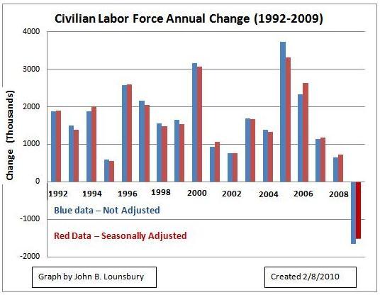
Note that two years 2005 and 2006 have the largest differences between seasonally adjusted data and non adjusted data. Curiously, the NSA data shows a larger labor force gain in 2005 and the reverse (SA larger) occurred for 2006. For the two years taken together, the sum of the NSA data and the SA data are nearly equal. I have no rationale to offer for this situation.
The following graph shows the SA and NSA data for employment. The agreement observed between SA data and NSA data is similar to the labor force graph. For employment, 2005 shows a very large difference between adjusted and unadjusted data and 2006 had less difference (than 2005), but is also larger than the other years.

The table below summarizes the agreement/disagreement between SA and NSA data. Data for 16 years falls within +/- 0.1% agreement between the annual changes calculated using NSA data and SA data. However, the data for 2005 and 2006 is much different. I would like to know the DOL explanation for this.

The disagreements falling within +/-0.1% (except for the renegade 2005-2006 interval) corresponds to an error equal to or less than the order the order of +/-120,000 to +/-150,000. Since the annual changes are calculated by the differences between two numbers each with an uncertainty of +/-300,000 the small disagreements between NSA and SA data indicate the seasonality adjustments are consistent from year to year and do not introduce bias.
Three of the four renegade data points fall in the range of +/-300,000 to +/-400,000, so those results are also within the range consistent with the uncertainty in the individual data points. The result for employment in 2005 is way outside what would be expected, of the order of 1% difference (+/-1.5 million). Again, I would like the DOL explanation for this.
Using Moving Averages
I have found it useful to smooth employment data using 4-month moving averages. An example is the following graph from last week’s article at TheStreet.com:
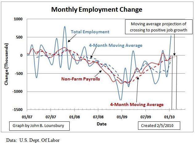
Moving averages smooth the data in a way that makes possible extrapolating forward from noisy data. The use of the 4-month moving average decreases the measurement error uncertainty present in the monthly data. The uncertainty in the moving average can be estimated by recognizing that the uncertainty is proportional to the standard deviation of the data sets. The equation for standard deviation of a data set is inversely proportional to the square root of the number of samples. See Appendix 3.
The 4-week moving average with each week having 60,000 data points is the equivalent of having 4 x 60,000 = 240,000 data points. The ratio is 4/1, with a square root of 2. If the uncertainty in the total population projected from a sample of 60,000 is +/- 300,000, then quadrupling the sample cuts the uncertainty regarding the entire population in half. The 4-week moving average has an uncertainty approximately +/-150,000.
Conclusions
There are a number of things necessary to avoid going crazy dealing with employment numbers.
- Recognize that a lot of what is published in the media reflects no understanding of what is significant and what is noise.
- Do not confuse the two different surveys and what is done with data from each.
- Recognize that moving averages are often needed to make any short term extrapolations.
- Don’t obsess on political interference with employment data. I can find no evidence that there is any political manipulation of the surveys or data analysis.
- Accept that adjustment model errors do occur (like the birth/death model) that require later correction. I have found no adjustments with modeling errors in the data that is used to determine employment, unemployment, the rate of unemployment, the civilian labor force and the number not in the labor force.
- Realize that the criteria for excluding people not working from the ranks of the unemployed and the civilian labor force is something worth reexamining.
I’m sorry to disappoint those that want to find a conspiracy theory. I am always looking for such, but I don’t find it in the Dept. of Labor or the Bureau of Labor Statistics. I would like to see more of the raw data published, but the model adjustments are published monthly so the raw data can be back calculated. And, I do believe that there are more ways to use the data in a productive way than has been done to date. One example is the proposal to use a standard work week and hours worked to define the level of unemployment, as published here.
Appendix 1: DOL Discussion of Confidence Intervals
A discussion of confidence intervals can be found here.
For example, the confidence interval for the monthly change in total nonfarm employment from the establishment survey is on the order of plus or minus 100,0001. Suppose the estimate of nonfarm employment increases by 50,000 from one month to the next. The 90-percent confidence interval on the monthly change would range from -50,000 to +150,000 (50,000 +/- 100,0002). These figures do not mean that the sample results are off by these magnitudes, but rather that there is about a 90-percent chance that the "true" over-the-month change lies within this interval. Since this range includes values of less than zero, we could not say with confidence that nonfarm employment had, in fact, increased that month. If, however, the reported nonfarm employment rise was 250,000, then all of the values within the 90-percent confidence interval would be greater than zero. In this case, it is likely (at least a 90-percent chance) that nonfarm employment had, in fact, risen that month. At an unemployment rate of around 5.5 percent, the 90-percent confidence interval for the monthly change in unemployment as measured by the household survey is about +/- 280,000, and for the monthly change in the unemployment rate it is about +/-0.19 percentage point.
Appendix 2: Seasonality Adjustments
The following is a statement from Chapter 1, BLS Handbook of Methods
Over the course of a year, the size of the Nation’s labor force, the levels of employment and unemployment, and other measures of labor market activity undergo sharp fluctuations due to such seasonal events as changes in weather, reduced or expanded production, harvests, major holidays, and the opening and closing of schools. Because these seasonal events follow a more or less regular pattern each year, their influence on statistical trends can be eliminated by adjusting the statistics from month to month. These adjustments make it easier to observe the cyclical and other nonseasonal movements in the series. In evaluating changes in a seasonally adjusted series, it is important to note that seasonal adjustment is merely an approximation based on past experience. Seasonally adjusted estimates have a broader margin of possible error than do the original data on which they are based, because they not only are subject to sampling and other errors but also are affected by the uncertainties of the seasonal adjustment process itself.
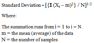
Appendix 3: Standard Deviation
The standard deviation of a data set is defined by the following equation:
Disclosure: No stocks mentioned.