Faltering Thursday – The Sell-Off Gains Momentum

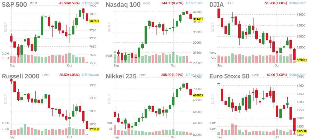
Those charts are kind of ugly, aren’t they?

Keep in mind there are about a dozen stocks holding up the Nasdaq 100 and the S&P and the Dow includes AAPL, AMZN, CAT, CSCO, GOOGL, MSFT, NVDA and CVX and JPM yet it is STILL down 4% in for the month! The Russell is down 6% and Europe is down 5% – yet people keep asking me why I’m being so cautious? 

It’s easy to make money – we just did our $700/Month Portfolio Review and our CAG spread has 308% upside potential, M has 159% upside potential, PFE (our 2026 Trade of the Year) still has 156% upside potential, PINS has 128% upside potential (2 years) and UNG has 240% upside potential and all of them should hit their goals in a flat or up market. 

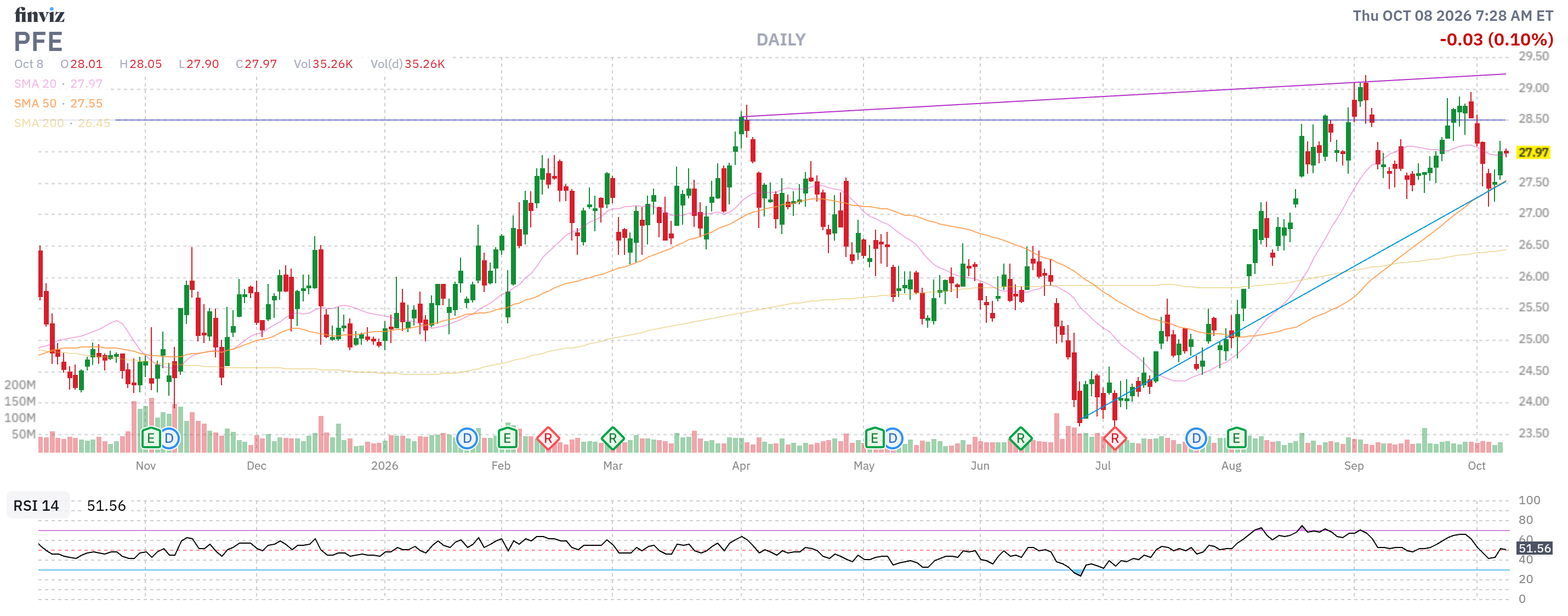
Our Trade of the Year isn’t the stock that will go up the most but the stock we can design an options spread around that is most likely to return 300% and, on Dec 16th, 2025 – our official trade idea for PFE was:

• • • • Buy 50 PFE 2028 $25 calls for $4 ($20,000)
      • Sell 40 PFE 2028 $32 calls for $1.90 ($7,600)
      • Sell 25 PFE 2028 $25 puts for $4.10 ($10,250) 
      • Sell 20 PFE March $26 calls at $1.55 ($3,100)
      • Sell 20 PFE March $25 puts at $1.22 ($2,440) 

That’s a net $3,390 CREDIT on the $35,000 spread so there’s $38,390 (1,132%) upside potential at $32 and we sold $5,540 (163%) worth of premium in the first quarter. 7 more sales like that generates a potential $38,780 (1,143%) – MORE THAN THE SPREAD! You can see why we feel this trade has such a high likelihood of returning 300%.  We are being aggressive with the short puts, risking an assignment of 4,500 shares at $25 ($112,500) so keep in mind it’s not NECESSARY to sell that many puts unless you REALLY want to own 4,500 shares at $25 but, with a forward p/e of 8.26 and a $1.70 (6.8%) dividend – why would I NOT want to own 4,500 shares?  

PFE closed at $26.97 in March (20th) so we had to pay 0.97 ($1,940) back to the short caller and the short puts expired worthless (because we were over the target) so we had collected $5,540 and we paid back $1,940 for a net profit of $3,600 – over 100% of our initial credit collected in one quarter!  

Of course we do sales every quarter in our Live Member Chat Room but, even if you are a cheapskate who only reads the free stuff, you started with a $3,390 credit on Dec 16th and then another $3,600 drops into your pocket on March 20th and now the spread is: 

• • • • 50 PFE 2028 $25 calls for $4.60 ($23,000)
      • 40 PFE 2028 $32 calls for $1.55 ($6,200)
      • 25 PFE 2028 $25 puts for $1.85 ($4,625) 

That is now net $12,175 PLUS the initial $3,390 credit PLUS the $3,600 in premium sales is net $19,165, which is already 565% higher than our initial credit. The short puts gave us an obligation to buy 2,500 shares of PFE for $25 ($62,500) but, in a Portfolio Margin Account (Schwab) – the buying power effect is only $6,536.25:

Now, this is a $35,000 spread and still only net $12,175, so there is STILL an upside potential of $22,825 (187%) PLUS we can still sell short-term put and call premium each quarter to generate another $12,000 (100%) of income so this is STILL, AFTER we’ve ALREADY made 565% – GOOD FOR A NEW TRADE!  

So, we are NOT worried about making money in an up market or a flat market – we are ONLY worried about LOSING money in a market correction. And why do they call them corrections? Because the market moves back to the CORRECT pricing for stocks – not these AI bubble-driven highs…  

But you can’t make money if you don’t have money – so we are PROTECTING our portfolios and erroring on the side of caution into earnings (which begin next week) so we can see the Q3 results and the Q4 guidance and decide how much of our CASH!!! (well over 50% of our portfolios at the moment) we want to deploy into the end of the year.  

And the funny thing about it is we’re NOT options traders. At PhilStockWorld, we are FUNDAMENTAL investors who, after identifying strong VALUE stocks, identify options spreads that give us both leverage and hedges going forward: 

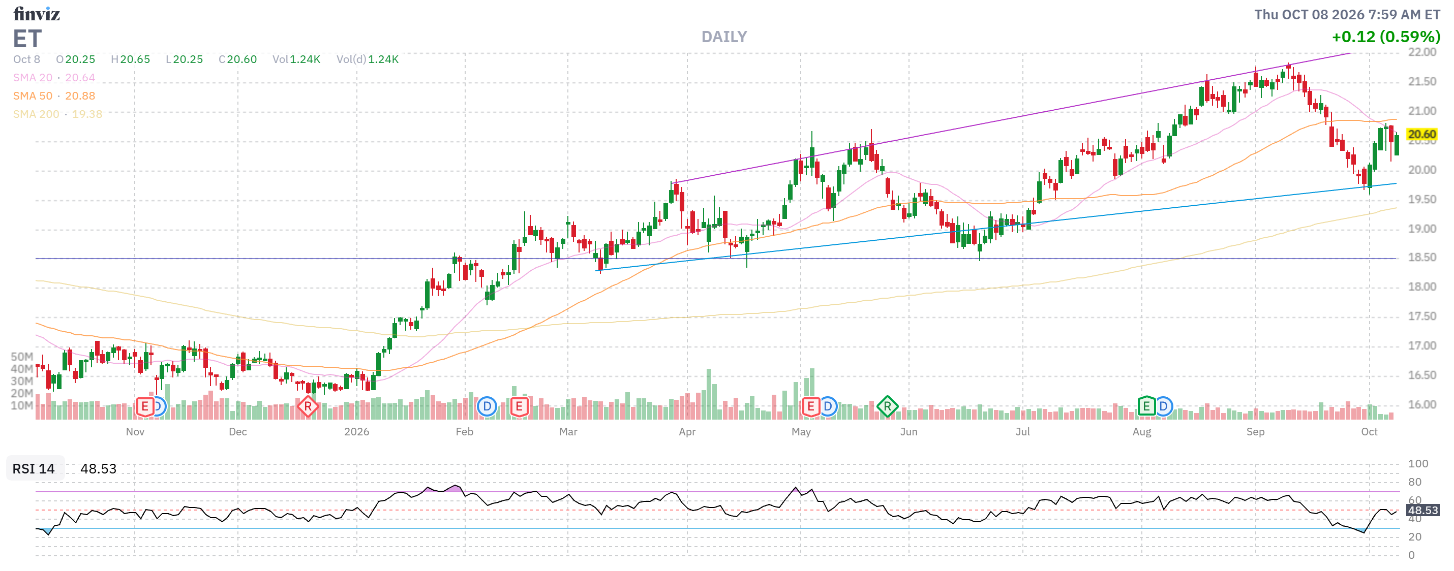
Our other Trade of the Year finalists last December were: Energy Transfer (ET):

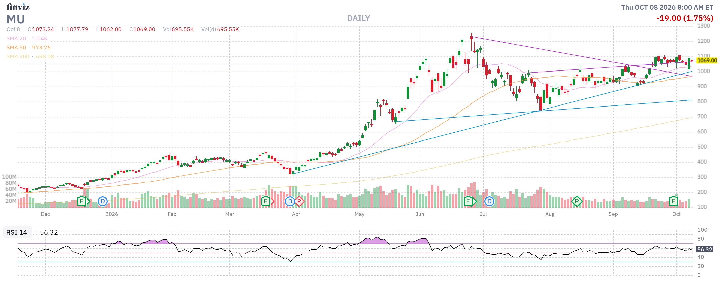
Micron (MU): 

And PPL Corp (PPL):  

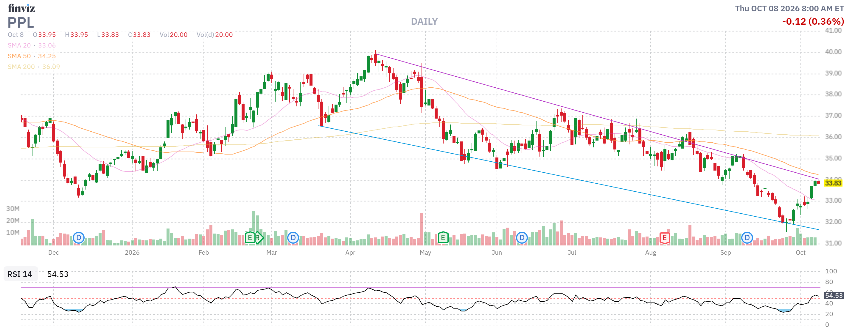
PPL has been disappointing as a stock but HERE is the key lesson to absorb. NOT that PFE made money or MU went to the moon but PPL, which is DOWN since December, had the following trade idea:

• • • • • Buy 25 PPL 2028 $30 calls for $5.70 ($14,250) 
        • Sell 20 PPL 2028 $40 calls for $2.70 ($5,400) 
        • Sell 15 PPL 2028 $35 puts for $4 ($6,000) 
        • Sell 10 PPL April $35 calls for $1.15 ($1,150) 
        • Sell 10 PPL April $33 puts for $1.10 ($1,100) 

That is net $600 on the $25,000 spread so there’s $24,400 (4,066%) of upside potential and we’ve collected $2,250 (375%) in premium sales for Q1 but it’s 122 days out of 766 we have to sell so let’s call it 6 more sales of $2,250 would be $13,500 (2,250%) of potential premium income while we wait.  Not bad… 

PPL was $39.02 on April 17th (expirations) so we had to pay to the short caller back $4,020 for a net LOSS of $1,770.  Of course we turned around and sold July puts and calls (success) and Oct puts and calls (on track) but, again, assuming you are too cheap to subscribe – the rest of the trade is now:  

• • • 25 PPL 2028 $30 calls for $7.70 ($19,250) 
    • 20 PPL 2028 $40 calls for $1.30 ($2,600) 
    • 15 PPL 2028 $35 puts for $3.50 ($5,250) 

That’s now net $11,400 and, even less the $1,770 loss on our first round of premium sales – that’s still net $9,630, which is up $9,030 (1,505%) against our $600 cash outlay! Aren’t you glad you didn’t subscribe? Look at all the taxes you would have to pay on these profits! 

$40 is still our Jan 2028 target and that would be a $25,000 spread so there is still $13,600 (119%) upside potential on the main spread and we could sell 10 April $35 calls for $1.50 ($1,500) and 10 April $33 puts for $1.50 ($1,500) and there’s a $3,000 (26%) bonus collected using 190 days out of 470 so likely we get ANOTHER chance to sell $3,000 in premium in October as well – so still a nice little trade – AND THIS IS THE ONE THAT DIDN’T WORK OUT!  

You should not be scared of options – you should be terrified of NOT knowing how to use them properly – ESPECIALLY as we head into a far more dangerous, choppy market in 2027!  

The “Be the House” Philosophy: Structural Investing vs. Speculative Gambling

Core Pillars of Structural Trading

┌─────────────────────────────────────────────────────────────────┐
│                    THE HOUSE OPERATING SYSTEM                   │
├───────────────────┬──────────────────────┬──────────────────────┤
│ 1. MACRO BASELINE │ 2. ASYMMETRIC DESIGN │ 3. COST BASIS DECAY  │
│ Valuation floors  │ High-upside spreads  │ Harvesting premium  │
│  & hard reality   │  subsidized by puts  │  to grind risk to $0 │
└───────────────────┴──────────────────────┴──────────────────────┘

1. Ruthless Macroeconomic Anchoring

2. Asymmetric Architecture (The Multi-Leg Framework)

3. Trapping Time via Options Physics

Defensive Mechanics: Pre-Planning for the “Losers“

To understand how “The House” operates, you have to look past the stock price and look at the internal mechanics of an options contract. In structural investing, options are not directional bets—they are financial instruments governed by Options Physics.

The two most critical forces in this engine are Delta (the price mover) and Theta (the clock). By understanding how these two forces interact, you can mathematically trap time decay and neutralize directional anxiety.

---

⏳ 1. Theta Decay: The Casino’s Edge

Theta represents the rate at which an option’s value declines as it approaches its expiration date. This is the mathematical embodiment of time decay.

• • The Buyer’s Disadvantage: When a retail speculator buys an option, the clock is their enemy. Every single day that passes, the value of that option ticks downward, melting away like an ice cube.
  • The House Advantage: When you sell (or write) an option, you become the casino (0:38). Theta decay shifts from a punishing cost into your primary revenue stream. You are collecting premium upfront, and time is working to grind the value of that contract down to zero so you can keep the profit (5:51).

The Theta Curve Acceleration

Theta decay is not linear. It follows an exponential curve that behaves differently based on how much time is left on the clock:

Option Value
  ▲
  │   ● (90 Days Out: Slow, steady decay)
  │    \
  │     \
  │      ● (60 Days Out)
  │       \
  │        \● (30 Days Out: The Cliff)
  │         └───► ● (Expiration: Value hits $0)
  └──────────────────────────────────────────► Time to Expiration

 

• • Long-Term Options (LEAPs): If you sell an option that expires in two years, the daily time decay is incredibly slow. The option retains its value for a long time.
  • Short-Term Options: As an option enters its final 30 to 45 days before expiration, Theta decay accelerates dramatically. The value drops off a cliff.
  • The Strategy: As highlighted in the video, “The House” exploits this curve by purchasing long-dated options (where time decay is slow and harmless) and systematically selling short-term options against them (where time decay is fast and aggressive). You are effectively buying slow-melting ice and selling fast-melting ice.

---

📊 2. Delta: The Risk Equalizer

Delta measures how much an option’s price is expected to move for every $1.00 change in the underlying stock. It is typically expressed as a decimal between 0.00 and 1.00 for calls (and 0.00 to -1.00 for puts).

• • The Probability Proxy: In practical trading, Delta is frequently used as a rough, real-time estimate of the probability that an option will expire in-the-money. A Delta of 0.40 means the option has roughly a 40% chance of finishing in-the-money at expiration.
  • The Directional Exposure Tracker: Delta tells you exactly how much directional exposure your account has. If you own 100 shares of stock, you have a Delta of 1.00 (you gain $100 if the stock goes up $1, and lose $100 if it drops $1). If you own a call option with a 0.50 Delta, your position behaves exactly like owning 50 shares of stock at that exact moment.

---

🧮 3. Unlocking “Options Physics“: Delta-Neutral Theta Trapping

The ultimate mastery of structural trading happens when you use Delta and Theta together to neutralize market volatility.

 

When retail traders see a stock rally and blow past the strike price of an option they sold, they panic because their upside feels “capped“. The video highlights a sophisticated structural adjustment using HPQ to show how the House handles this:

1. 1. The Matching Engine: If your short-term sold option is getting challenged, you can buy or hold a long-term option where the Deltas perfectly match (e.g., a long call with a 0.42 Delta and a short call with a 0.43 Delta).
   2. The Result: Because the Deltas are nearly identical, a sudden, erratic swing in the stock price changes the value of both options equally. The directional risk is effectively neutralized or “insulated.”
   3. The Trap: Even though the stock price movements are canceling each other out, the Theta decay is not equal. The short-term option is bleeding value to time decay exponentially faster than the long-term option.

You have created a structure where you don’t need to know where the stock is going. You have built a mathematical cage that traps time, allowing you to harvest consistent gains while remaining completely detached from day-to-day market anxiety (0:44).

 

To see how the “House” operates over a prolonged period, let’s track a systematic, step-by-step mathematical example using Transocean(RIG).

We will assume the Worst-Case Planned Risk Scenario from the video: the macro thesis remains solid, but the stock price drops and you are assigned 2,000 shares at $5.00 per share.

 

Here is exactly how the math grinds your risk down to zero over time, contract by contract, cycle by cycle.

---

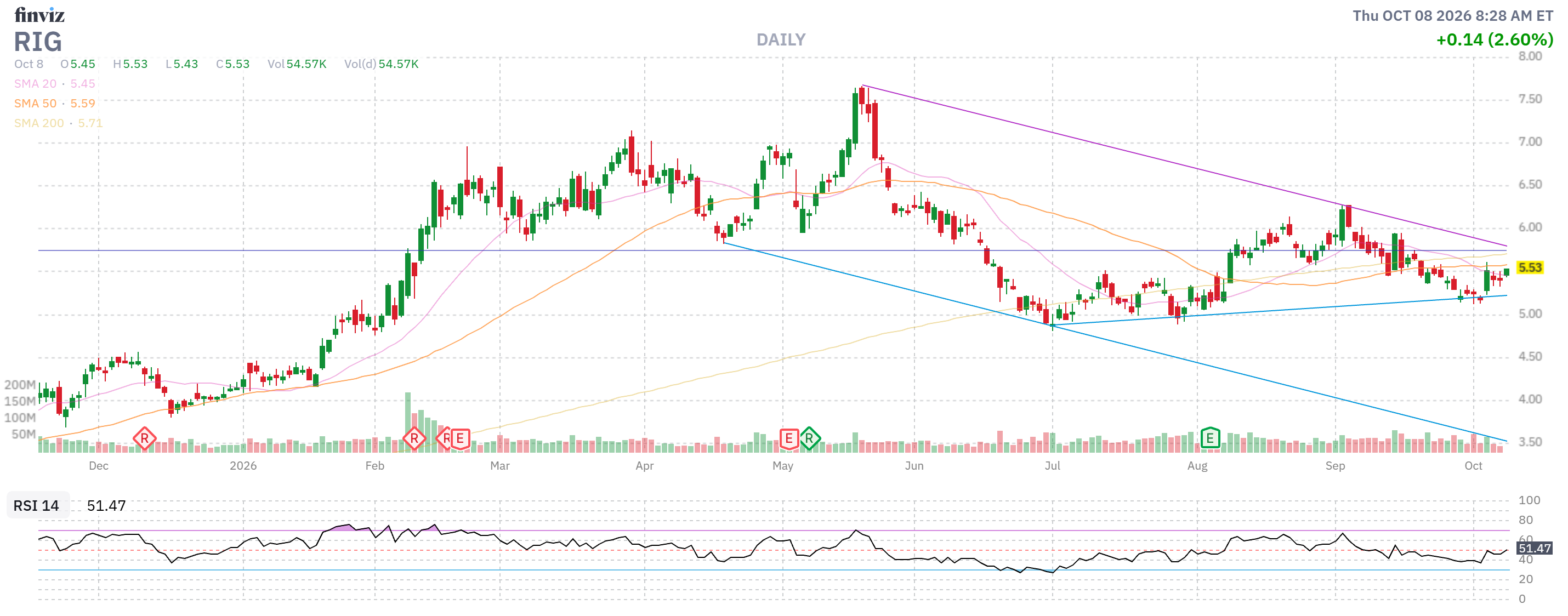
🏁 Step 0: The Baseline Assignment (Month 0)

The market has dropped, your short puts have expired in-the-money, and you are forced to buy the stock.

• • Shares Owned: 2,000 shares of RIG.
  • Capital Layout: $10,000.
  • Initial Net Cost Basis: $5.00 per share.

(Note: In reality, your starting basis would be slightly lower because of the $100 net credit collected when you first opened the trade, but we will keep the math clean at exactly $5.00 to show the power of the covered call engine alone).

---

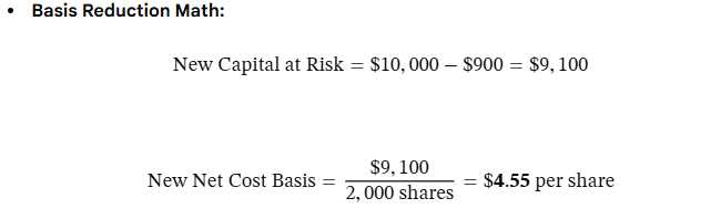
🔄 Cycle 1: The Initial Harvest (Months 1–6)

Instead of waiting and hoping for RIG to climb back up, you immediately pivot to generating cash. You look out 6 months and sell 20 Covered Calls at the $5.00 strike (matching your 2,000 shares).

 

Let’s assume you collect a conservative premium of $0.45 per share.

• • Upfront Cash Collected: $2,000 \times \$0.45 = \mathbf{+\$900}$
  • Account Dynamic: Your broker deposits $900 directly into your cash balance.

---

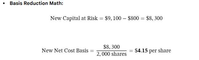
🔄 Cycle 2: Compounding the Grind (Months 6–12)

Six months have passed. Transocean’s stock has hovered sideways around $4.20. Because it stayed below $5.00, the covered calls you sold expire completely worthless. You keep the $900, and you still own all 2,000 shares.

 

You rinse and repeat. You sell another 6-month covered call at the $5.00 strike, this time collecting $0.40 per share.

• • Upfront Cash Collected: $2,000 \times \$0.40 = \mathbf{+\$800}$
  • Account Dynamic: Another $800 in raw cash hits your account.

---

🔄 Cycle 3: The Intrinsic Inflection Point (Months 12–18)

It has now been one year. Your total cash generated from premium harvesting is $1,700 ($900 + $800). The second round of calls expires worthless. You step up to the plate to sell a third round of 6-month contracts, collecting $0.35 per share.

 

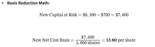
• • Upfront Cash Collected: $2,000 \times \$0.35 = \mathbf{+\$700}$

---

📊 The Mathematical Shift: Visualizing the Break-Even Evolution

Look at what has happened to your risk profile after just 18 months of operating as the House, even though the stock price never went up:

 Price Per Share
  ▲
$5.00 ├─────────────────────────────────────────► Your Initial Cost Basis
      │
$4.50 ├───────────┐ New Cost Basis (Cycle 1)
      │           │
$4.00 ├───────────┼───────────┐ New Cost Basis (Cycle 2)
      │           │           │
$3.50 ├───────────┼───────────┼───────────┐ New Cost Basis (Cycle 3: $3.80)
      │           │           │           │
      └───────────┴───────────┴───────────┴─────► Time (Cycles)

---

🏁 The Payoff Scenarios at Month 18

Because you have relentlessly lowered your net cost basis to $3.80, the psychological anxiety of the trade is entirely gone. Let’s look at how the mathematics protect you in three different market directions:

Scenario A: The Stock Stays Flat or Slumps ($4.00)

A traditional retail investor who bought at $5.00 is down -$1.00 per share and staring at a -$2,000 paper loss. You, however, are net profitable. Because your basis is $3.80, you are actually up +$0.20 per share (+$400 total value). You simply let the options expire and sell Cycle 4 to keep lowering the basis further.

Scenario B: The Stock Recovers and Triggers the Call ($5.50)

RIG catches a macro tailwind and rallies to $5.50. The person who bought your $5.00 calls exercises their right to buy your shares.

• • You are forced to sell your shares at $5.00, collecting $10,000.
  • Your actual capital at risk left in the trade was only $7,600.
  • Your Final Profit: $10,000 – $7,600 = $2,400 – A 24% return on your original asset layout, manufactured while the stock barely moved past your original buy price).

Scenario C: The Multi-Year Long Grind (Grinding to $0.00)

As noted in the video, if you expand this horizon over an extended macro cycle (using multi-year options or sequential short-term rolls), the cumulative premiums collected can eventually cross the $10,000 threshold. Once you collect $10,000 in cash premiums, your net cost basis becomes $0.00. You own 2,000 shares of a major infrastructure company entirely for free and every single dividend or subsequent call option sold from that day forward is 100% pure profit.

 

Stop trading at the mercy of the market. STOP being the hapless gambler and join PhilStockWorld – where we will teach you (and we’ve been doing it for 20 years – so we’re very confident) to: 

Be the House – NOT the Gambler!  

This video is from 2013!